Model Building with Simulink

This tutorial is the first in a series of tutorials that discuss the essential features of Simulink as required to model, simulate and analyse dynamic systems.

Specifically this tutorial covers topics related to building models. The topics are broken into the following sections,

1. The Library Browser.
2. Opening a New or Existing Model.
3. Inserting Blocks.
4. Connecting Blocks.
5. Modifying Block Parameters.

See the Simulink Essentials - Building and Simulating Models page for links to tutorials discussing how to simulate a model once it has been built and view signals created in the model. Other tutorials discussing Simulink and its applications for model based design are available on the Software Tutorials page.

The Library Browser

Blocks to be used within a model are typically obtained from libraries. (A library is simply a collection of existing blocks.) The standard Simulink libraries are conveniently displayed in the Simulink Library Browser. The Library Browser may be opened in several different ways, the most common of which are to either press the Simulink button on the MATLAB Desktop (i.e. the main MATLAB user interface), or by typing simulink at the MATLAB command prompt. These approaches are shown in Figure 1

Figure 1: Opening the Library Browser.

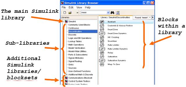
The open Library Browser is shown in Figure 2. On the left hand side is a tree view of the available libraries. The main Simulink libraries appear at the top of the tree view, while custom libraries -- that may be user created or purchased separately -- appear below it.

Libraries may consist of sub-libraries. If this is the case then the sub-libraries, and the blocks within the libraries, are viewed by opening the tree structure in the left pane and viewing the contents in the right pane.

Figure 2: Looking at Libraries Displayed in the Library Browser.

Opening a New or Existing Model

There are many different ways to open an existing Simulink model. This may be done for the purpose of either viewing the model, simulating the model, or for making modifications to the model. Figure 3 shows several of the more common ways that an existing model may be opened. These include using the File→Open pull-down menu; double-clicking on the name of a model in the Current Folder; and typing the name of the model at the MATLAB command prompt.

Figure 3: Opening an Existing Model.

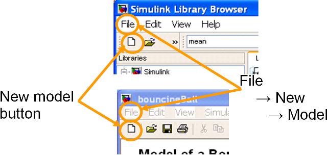
Similarly there are several different ways that a new model can be opened. The two most common approaches are shown in Figure 4: using the File→New→Model pull-down menu; and pressing the New Model button on the menu-bar of either the Library Browser or an existing model.

Figure 4: Opening a New (i.e. Empty) Model.

Inserting Blocks

Blocks are inserted into a model (from a library) by using a standard drag-and-drop operation with the left mouse button. Depress the left mouse button on a block within a library, then drag the mouse across to the model into which it needs to be inserted, and then release the left mouse button.

Alternatively a block may be added to a model by right clicking on it in the Library Browser and selecting the Add to MODELNAME option, where MODELNAME is the name of the model into which the block is to be added.

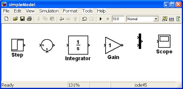
Figure 5 shows an example of a model that has had 6 blocks added to it. The Step block has been obtained from the Sources library; the Sum and Gain blocks have been obtained from the Math Library; the Integrator has been obtained from the Continuous library; the Mux block has been obtained from the Signal Routing library and the Scope block has been obtained from the Sinks library.

Figure 5: Blocks Inserted Into a New Model.

Once a block has been added to a model there are a multitude of operations that may be performed on it. These include operations that define the topology of the model and how the block behaves during simulation. Two such operations described later in this tutorial are,

1. Connecting/disconnecting it to/from other blocks.
2. Modifying block parameters.

There are also many purely cosmetic changes (i.e. changes that do not effect the simulation results) that may be used to make the model more readable and hence understandable. These include,

1. Renaming.
2. Repositioning.
3. Copying.
4. Resizing.
5. Rotating and flipping.
6. Changing the foreground and background colors.

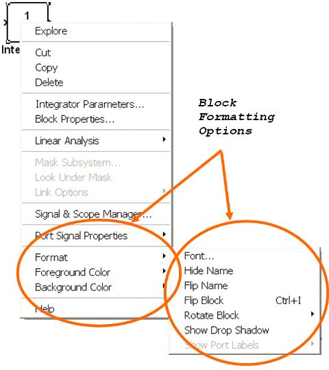
The above operations are achieved by either right clicking on the block of interest and selecting the appropriate formatting operation (this is shown in Figure 6) or using standard mouse operations to select and then drag or resize the block.

Figure 6: Options for Formatting a Block.

Connecting Blocks

Once a block is in a model it (typically) needs to be connected to other blocks. This is achieved by drawing a line between the outputs and inputs of the appropriate blocks. These lines are called signals.

To create a signal depress the left mouse button over the outport of the source block (i.e. the block where the signal will originate), then drag the mouse to the inport of the destination block (i.e. the block where the signal will terminate), then release the mouse button. By default Simulink will draw a large black arrowhead on the signal indicating the direction of data flow.

There are several aspects of drawing signals that are worth highlighting,

• As the mouse is being dragged Simulink draws the signal, thus providing visual feedback about where the signal will appear.
• Signals may be dropped anywhere in the model, not just at block inports. This can be useful when needing to draw signals that go around other blocks.
• Signals that are not connecting blocks are drawn in red, thus providing visual feedback that a signal is not connected. This can be useful for debugging purposes (as it is easier to see whether a signal has been erroneously not connected).
• Signals may be drawn from either the source block to the destination block (as described above) or from the destination block to the source block. Since a signal may only originate at an outport and only terminate at an inport Simulink will draw the arrow head (that indicates the direction of signal flow) in the correct direction.
• Sometimes signals need to be branched so that they can flow into multiple destination blocks. A signal branch is created by depressing the right mouse button on an existing signal, then dragging away from the signal, then releasing the mouse button.

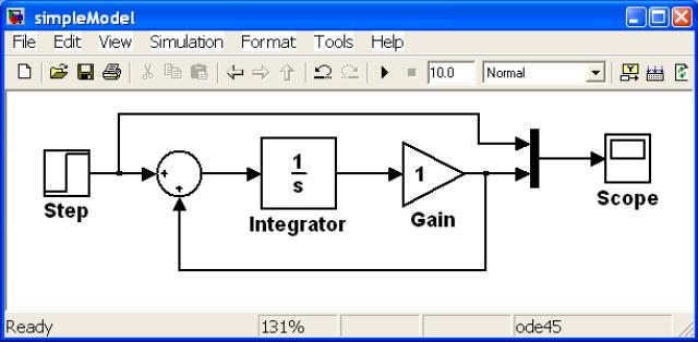
Figure 7 shows a simple model where all of the blocks have been connected by signals. Note the arrow heads indicate signal flow and the branching of two of the signals to enable them to feed into multiple blocks.

Figure 7: Blocks Connected and Showing Signal Flow.

Modifying Block Parameters

Typically a block taken directly from a library will not be configured exactly as required. For example the Gain block has a default gain of 1, which is rarely going to be the value required in a model (if it was then a Gain block wouldn’t be required at all as a gain of 1 is superfluous).

The parameters of a block are viewed (and modified) by double-clicking the left mouse button on a block to open its Block Properties dialog. The Block Properties dialog for both the Sum block and the Gain block is shown in Figure 8.

Figure 8: Block Properties Dialog Box for the Sum block (left) and the Gain block (right).

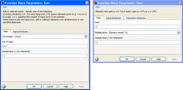
For the model considered in this tutorial two block parameters are changed. Firstly the List of Signs property of the Sum block has been changed from “|++” to “|+-” (without the quotes) thus converting it to a subtraction operator. And secondly the Gain parameter of the Gain block has been changed from 1 to 2. This is shown in Figure 9.

Figure 9: Model with Modified Sum and Gain Block Parameters.

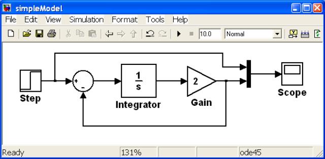
This tutorial has discussed topics related to constructing Simulink models. The model constructed implements a simple first order continuous time transfer function, and when simulated allows the step response of the transfer function to be visualized.

Simulating Models is the topic discussed in the next tutorial in this series, while other Simulink tutorials are available on the Software Tutorials page.

Back To Top | Simulink Tutorials