Interfacing Simulink with MATLAB
Simulink, being an add-on product to MATLAB, is very tightly integrated with MATLAB.
Although rarely done, it is possible to build a Simulink model from MATLAB code without ever using the Simulink user interface. This is achieved using the MATLAB-Simulink API (application program interface) commands.
More commonly, MATLAB is the environment used to pre- and post-process model parameters and signal data used in or generated by Simulink. This tutorial discusses some of the different ways that MATLAB and Simulink interact. The topics covered are,
- Specifying Model Parameters.
- Workspaces.
- Inputting Signal Data.
- Outputting Signal Data.
- Simulating from the MATLAB Command Line.
The model used throughout this tutorial is called simpleModel. It is constucted in the tutorial Simulink Essentials - Building, Simulating and Visualizing Models.
Other tutorials discussing Simulink and its applications for model based design are available on the Software Tutorials page.
Specifying Model Parameters
The gain in the transfer function modeled by the simpleModel developed in the tutorial Simulink Essentials - Building, Simulating and Visualizing Models has been hard-coded to have a value of 2. However the model can be used to model a generic first order transfer function, i.e. it can be used to simulate the step response of a transfer function with an arbitrary gain.
Rather than give the gain a specific (hard-coded, numeric) value, it is much better to parameterize it, i.e. to put the name of a MATLAB variable as the gain value. This is shown in Figure 1. More generally all model and block parameters should be defined as variables.
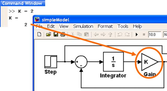
One of the first things Simulink does when the simulation is started is inspect the model and determine what parameters it needs for the simulation to run correctly. One of the places it looks for parameter values is the MATLAB Workspace. In the above case the variable K has been defined in the MATLAB Workspace and Simulink will obtain the value for K -- in this case 2 -- and use it for this simulation run.
If the step response of a transfer with a different gain is required then K can be redefined in the MATLAB Workspace and the simulation executed again.
Parameterization isn't too critical for very simple models such as simpleModel. The gain only appears once in the model and its value would be easy to change in the model itself. However as models become larger and more complex, and the same parameter is used in multiple places in a model, it becomes much more important to use a parameterized model. In this way the value of a gain (or any other model parameter) can be changed in one place (i.e. the MATLAB Workspace) and the new value will be used everywhere that the parameter is used in the model.
Workspaces
The term Workspace is MATLAB terminology for memory allocated to store data. Each MATLAB funcion has its own workspace, or memory allocated for it to create and destroy its locally scoped variables.
In Simulink each model has access to two workspaces: the MATLAB Base Workspace; and the Model Workspace. Each model has its own Model Workspace.
When a parameterized model is intialized it must be given values for the parameters that it needs. The model first looks in its Model Workspace to determine if any of the required parameters are present, and if they are then those values are used. If any variables are not defined in the model’s workspace then Simulink will look for them in the MATLAB Base Workspace. If the same variable exists in both locations then the value in the model’s workspace takes precedence.
The Model Workspace is created, viewed and modified via the Model Explorer. The Model Explorer is opened using the View→Model Explorer pull-down menu (see Figure 2).
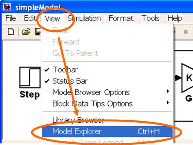
Once the Model Explorer is open then the model’s workspace can be viewed by selecting the appropriate node of the tree view down the left hand side. Figure 3 shows a value for the gain K being defined in simpleModel’s model workspace.
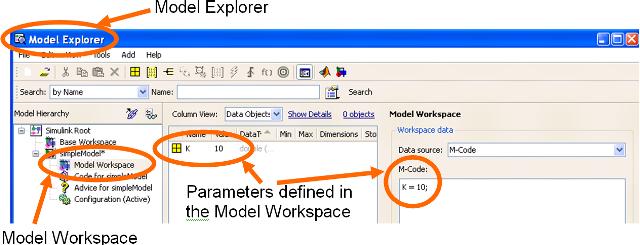
Note that there are several different ways to define the model workspace. Data may be defined either as m-code that defines the appropriate variables and gets automatically executed to create the variables, or within a .mat file that gets automatically loaded to create the variables.
Inputting Signal Data
Very often a user may wish to excite a model with externally created data. This may be artificially created or true test data from field tests.
If the data is stored in a .mat (binary MATLAB) data file then it may be imported into the model using a From File block.
If the data is in the MATLAB workspace then it may be imported using either a From Workspace block or an Inport Block. If an Inport block is used then the specific data to be used must be defined on the Data Import/Export pane of the Simulation→Configuration Parameters pull-down menu. (Initial values for the model states may also be specified on this panel.)
In all cases the data must be of a specific format. The data must be either a multicolumn matrix where the first column represents time (corresponding to the data in subsequent columns), or it must be a MATLAB structure data type with a field called time and another field with the signal data.
Figure 4 shows the simpleModel where the input Step block has been replaced by an Inport block. Figure 5 shows the Data Import/Export panel of the modified model’s Configuration Parameters dialog. To excite the model through the Inport block the Input check-box must be checked and appropriate data defined. In this case the input has been parameterized with the name of a MATLAB variable. Figure 6 shows one of the ways to define the required data in the MATLAB workspace. An appropriate structure is created that contains data defining a unit step function where the step takes place at t=1.
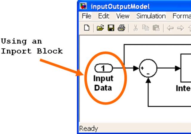

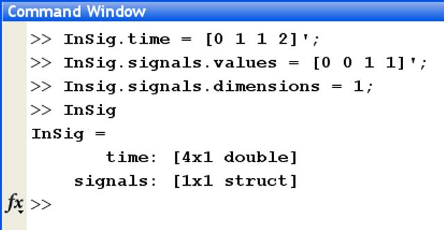
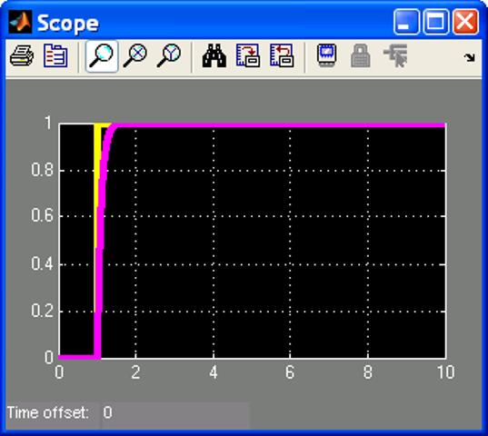
Figure 7 shows the output Scope when the model is simulated using the data fed through the Inport block. As expected it shows the step response of a first order transfer function.
Outputting Signal Data
Signal and state data can easily be saved at the completion of a simulation. (For reasons of efficiency data is not saved back to MATLAB during the simulation – only when the simulation is paused or stops.)
If the data is to be stored in a .mat (binary MATLAB) data file then it may be exported using a To File block.
It is more typical for signal data to be exported to MATLAB for post-processing. This may be achieved in numerous ways. The To Workspace block is a straight forward approach. However using an Outport (at the highest level of the model) or saving the data/signal being fed into a Scope block are more common approaches.
If an Outport block is used then the signal data is saved to the MATLAB Workspace. The name of the variable to create is define on the Data Import/Export pane of the Simulation→Configuration Parameters pull-down menu.
Several different formats for the saved data are available including a matrix, a structure with time and a structure without time. There are also options for automatically decimating the data (i.e. only saving every n-th time step) and only saving data for the last n number of time steps.
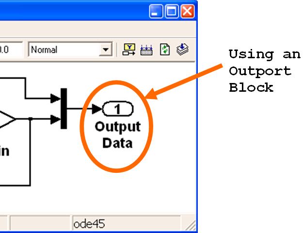
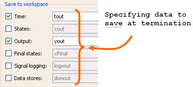
Figure 8 shows the simpleModel where the display Scope block has been replaced by an Outport block. Figure 9 shows the Data Import/Export panel of the modified model’s Configuration Parameters dialog. To save signal data through the Outport block the appropriate Save To Workspace check-boxes must be checked and appropriate variable names specified. In this case the model will save both the simulation time steps (in the variable tout) and the signal being fed into the Outport (in the variable yout).
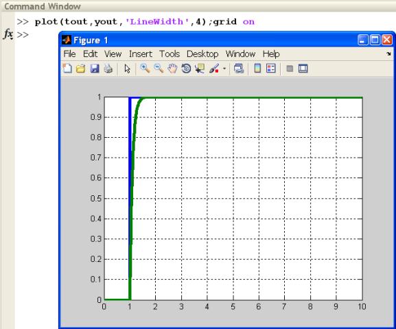
Once the simulation has been run the variables tout and yout will be saved to the MATLAB Workspace. Being standard MATLAB variables they may be post-process in any way the user wished to program. Figure 10 shows the appropriate MATLAB command to plot the data. As expected it shows the step response of a first order transfer function.
Simulating from the MATLAB Command Line
Once a model has been created and parameterized it can be simulated directly from the MATLAB command line, or more often from within a MATLAB function or script file. The function to do this is called sim.
The sim function has several different formats (shown in Figure 11) for allowing the user to override the model parameters set on the model’s Configuration Parameters dialog. In each of these cases the sim function returns a Simulink.SimulationOutput object that contains all of the data that the model would normally save to the MATLAB Workspace.
% Different syntaxes for the sim function
simOut = sim('model', 'ParameterName1',Value1,'ParameterName2', Value2...);
simOut = sim('model', ParameterStruct);
simOut = sim('model', ConfigSet);
The following code snippet will run the model called inputOutputModel ten times, each time with a different gain value. inputOutputModel is a modification of the simpleModel model (which is constucted in the tutorial Simulink Essentials - Building, Simulating and Visualizing Models) so that its output is saved to the MATLAB Workspace through an outport as discussed in the above Outputting Signal Data section and the gain is parameterized as discussed in the above Specifying Model Parameters section.
% Script to execute a Simulink model using the sim function
for K = 1:10
    data(K) = sim('inputOutputModel','ReturnWorkspaceOutputs', 'on');
end
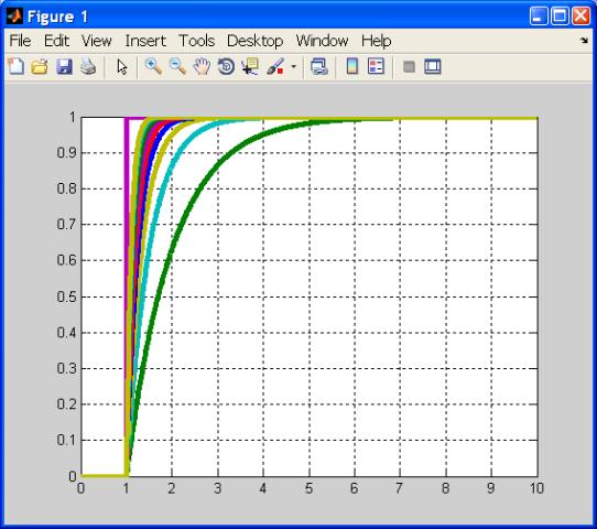
Note that each time through the loop in Figure 12 the value of the gain in the gain block changes and hence the rise time of the first order transfer function being simulated will change.
After the code in Figure 12 is executed the MATLAB Workspace will have the following variable defined in it,
>> data

1x10  Simulink.SimulationOutput array:
Each of the 10 elements of the Simulink.SimulationOutput object represents one of the 10 different simulation runs. Hence each element contains signal data showing a different rise time for the first order tansfer function being modeled.
The following code (see Figure 14) will extract the signal data saved to the Simulink.SimulationOutput object and overlay all 10 simulations on the same plot. The resulting plot is shown in Figure 15
% Script to Visualize the Simulation Data
for idx = 1:length(data)
    plot(get(data(idx),'tout'),get(data(idx),'yout'),'LineWidth',4);
    hold all
end
grid on
This tutorial has discussed topics related to interfacing a Simulink model to MATLAB. Other Simulink tutorials are available on the Software Tutorials page.