Simulating Multiple Asset Paths in MATLAB

This tutorial presents MATLAB code that generates multiple simulated asset paths which may be used in the Monte-Carlo approach to pricing options as discussed in the Monte-Carlo Methods tutorial. A tutorial for Generating Correlated Asset Paths in MATLAB is also available.

Note that the primary purpose of the code presented here is to show how to efficiently generate multiple asset paths. The code contains no error checking and as such it is not suitable for inclusion into a larger application without appropriate modifications.

MATLAB Function: AssetPaths

The following is code for generating a user specified number of simulated asset paths assuming the asset follows the standard log-normal/geometric Brownian motion model,

Equation 1: Stock Price Evolution Equation

function S = AssetPaths(S0,mu,sig,dt,steps,nsims)
% Function to generate sample paths for assets assuming geometric
% Brownian motion.
%
% S = AssetPaths(S0,mu,sig,dt,steps,nsims)
%
% Inputs: S0 - stock price
%       : mu - expected return
%       : sig - volatility
%       : dt - size of time steps
%       : steps - number of time steps to calculate
%       : nsims - number of simulation paths to generate
%
% Output: S - a matrix where each column represents a simulated
%             asset price path.
%
% Notes: This code focuses on details of the implementation of the
%        Monte-Carlo algorithm.
%        It does not contain any programatic essentials such as error
%        checking.
%        It does not allow for optional/default input arguments.
%        It is not optimized for memory efficiency or speed.

% Author: Phil Goddard (phil@goddardconsulting.ca)
% Date: Q2, 2006

% calculate the drift
nu = mu - sig*sig/2;

% Generate potential paths
S = S0*[ones(1,nsims); ...
            cumprod(exp(nu*dt+sig*sqrt(dt)*randn(steps,nsims)),1)];    

Example Usage

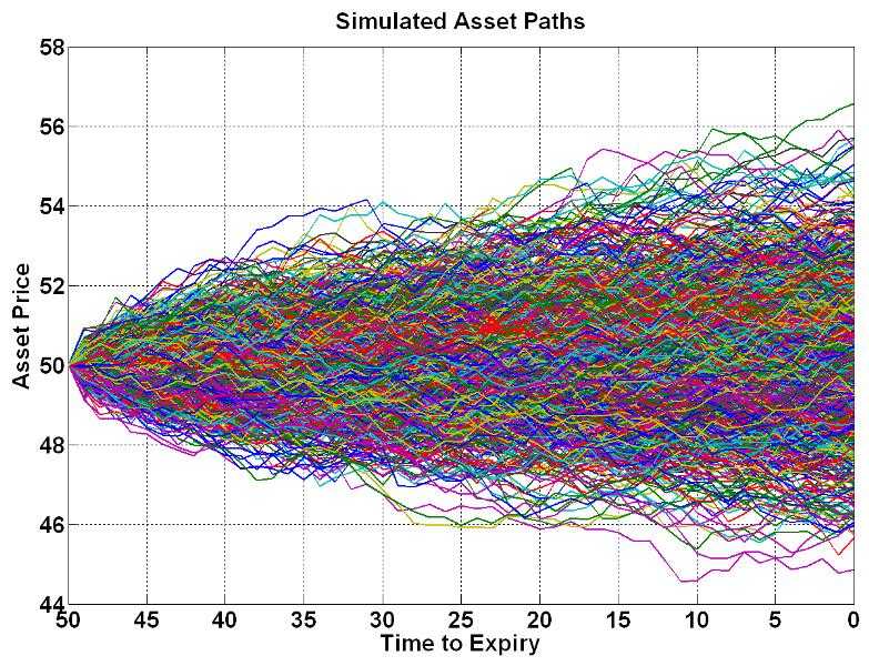
The following MATLAB code gives an example of how to use the function AssetPaths, including creating (and customizing) a plot showing the generated price paths.

% Script to price an Asian put option using a Monte-Carlo approach.

S0 =50;       % Price of underlying today
X = 55;       % Strike at expiry
mu = 0.04;    % expected return
sig = 0.1;    % expected vol.
r = 0.03;     % Risk free rate
dt = 1/365;   % time steps
etime = 50;   % days to expiry
T = dt*etime; % years to expiry

nruns = 1000; % Number of simulated paths

% Generate potential future asset paths
S = AssetPaths(S0,mu,sig,dt,etime,nruns);

% Plot the asset paths
time = etime:-1:0;
plot(time,S,'Linewidth',2);
set(gca,'XDir','Reverse','FontWeight','bold','Fontsize',24);
xlabel('Time to Expiry','FontWeight','bold','Fontsize',24);
ylabel('Asset Price','FontWeight','bold','Fontsize',24);
title('Simulated Asset Paths','FontWeight','bold','Fontsize',24);
grid on
set(gcf,'Color','w');

The resulting plot is shown below,

Figure 1: Multiple Monte-Carlo Generated Price Paths

An example of using the function AssetPaths to price Asian options is given in the Pricing an Asian Option in MATLAB tutorial.

Back To Top | Option Pricing