Simulink - Slip Control of a Quarter Car Model

This example presents a Simulink model of an automotive wheel slip control loop as might be used in a rudimentary ABS system. Although idealized equations are used, the overall model demonstrates many of the essential features of a good Simulink model.

Each of the individual components in the loop are discussed separately: a tire model; a standard quarter car model; a brake actuator; and a (PI) controller. The model for each component demonstrates a different feature of Simulink: the tire model shows how to implement a simple algebraic equation (that contains no state memory); the quarter car model shows how to implement non-linear continuous time equations; the actuator model shows how to handle time delays; while the controller shows how to implement discrete time difference equations.

Since the quarter car model and actuator are modeled in continuous time, while the controller is implemented in discrete time, the developed model is also a good example of how to implement hybrid continuous-discrete systems within Simulink.

The example is split into the following sections,

1. Overview of the Complete Model.
2. The Tire Model.
3. The Quarter Car Model.
4. The Actuator Model.
5. The Controller Model.
6. Simulating The Complete Model.

Other tutorials discussing Simulink and its applications for model based design are available on the Software Tutorials page.

Overview of the Complete Model

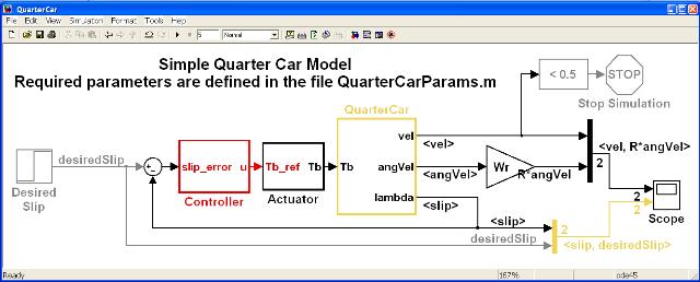
The control loop developed in this tutorial follows a very standard form. The controller, actuator and quarter car models are all in the feedforward path. The calculated wheel slip (which is to be controlled) is fed back and compared to a desired slip value, with the error fed into the controller. This is shown in Figure 1.

Figure 1: Quarter Car Slip Control Loop.

A zip file containing the model may be downloaded here.

Note that the model is fully parameterized. (Parameterizing models is discussed in the tutorial Specifying Model Parameters section of the Interfacing Simulink with MATLAB tutorial). All the parameters are created in the MATLAB workspace by executing the m-file QuarterCarParams.m which is done automatically when the model is opened. (This is achieved by specifying a PreLoadFcn for the model.)

Having the model parameterized enables the same model to be easily used for different vehicle types and configurations.

The model is only valid for vehicle speeds above 1–2 ms^-1. Hence it includes a Stop Block which stops the simulation when the speed drops below a small value – in this case 0.5 ms^-1.

The Tire Model

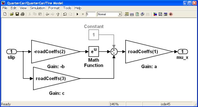
The tire model implemented in this example uses the standard Pacejk magic formula. In Pacejk’s model, the equation for the longitudinal friction coefficient μ_x is given by

Equation 1: Pacejk’s Magic Formula Tire Model.

where λ is the wheel slip, and the coefficients a, b and c change depending on the current road surface. This example assumes that the vehicle is being driven on dry asphalt and hence the coefficients are a = 1.28, b = 23.99 and c = 0.52.

The implmentation for the tire model equations is shown in Figure 2.

Figure 2: Tire Model Subsystem.

The Quarter Car Model

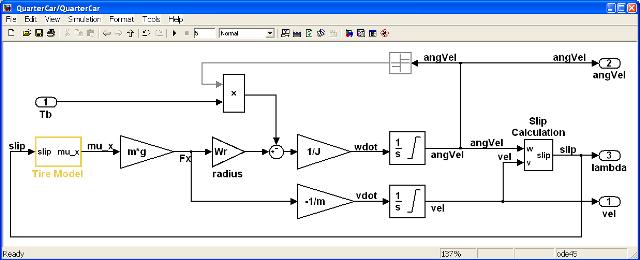
This example uses a standard set of equations for the dynamics of a quarter car. It contains two continuous time states, and is described by the set of non-linear equations in Equation 2,

Equation 2: Quarter Car Equations.

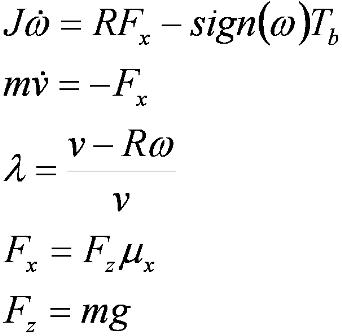
where ω > 0, ν > 0, and hence -1 < λ < 1.

The following table lists the definition of the notation used in Equation 2.

Name	Description	Value
ω	Angular Speed	Output Signal
ν	Longitudinal Speed	Output Signal
J	Inertia	1 Kg m2
R	Wheel Radius	0.32 m
Tb	Brake Torque	Input Signal
Fx	Longitudinal Force	Calculated
λ	Longitudinal Wheel Slip	Calculated
Fz	Vertical Force	Calculated
μx	Road Friction Coefficient	Calculated
m	Quarter Vehicle Mass	450 Kg
g	Gravitational Force	9.81 ms-2

Table 1: Notation for the Quarter Car Model.

The implementation of quarter car equations is shown in Figure 3.

Figure 3: Quarter Car Model Subsystem.

The Actuator Model

Actuator dynamics, and particular time delays, are often critical to the design of a sufficiently accurate control algorithm. This example uses a simple first order lag in series with a time delay to model the actuator. (In practice a second order model is almost always required, and often actuators have different responses when they are opening and closing, and hence need to be modeled in considerable more detail than is done here.)

The model for the actuator are given by Equation 3,

Equation 3: Actuator Equation.

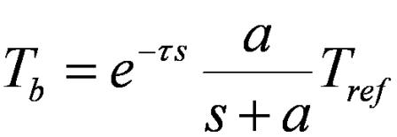
subject to the constraint that 0 < T_b < T_{b_sat}.

The following table lists the definition of the notation used in Equation 3.

Name	Description	Value
τ	Time Delay	0.05 s
a	Filter Pole Location	70
Tb_sat	Saturation	4000

Table 2: Notation for the Actuator Model.

The implementation of actuator equations is shown in Figure 4.

Figure 4: Actuator Model Subsystem.

Note that the first order lag (transfer function) has been implemented using an integrator, gain and summation/negation block rather than a Transfer Funtion Block (from the Continuous library). This has been done as the Transfer Function block does not allow vector signals as an input, but the current implementation does. Hence the model being developed can more easily be expanded to allow for 4-channels, i.e. one for each wheel on a four wheeled vehicle. A Transfer Function Block would preclude that from happening (without replacing the block).

The Controller Model

There are many different potential implementations for the controller. Here a simple PI (proportional–integral) controller has been shown to be adequate.

The implementation of controller is shown in Figure 5.

Figure 5: The Controller Subsystem.

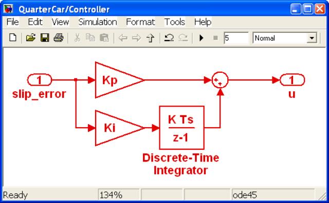
Note that the subsystem has been made atomic, and given a discrete sample rate of T_s = 5ms.

Controller gains that have been determined to work reasonably well for the configuration chosen here are K_p = 1200 and K_i = 100000.

Simulating The Complete Model

Once the model components have been implemented and connected, and the parameters defined, then the model may be simulated. (See the Simulating a Simulink Model tutorial to see how to execute a Simulink model.) The results for the current configuration are shown in Figure 6.

Figure 6: The Simulation Results.

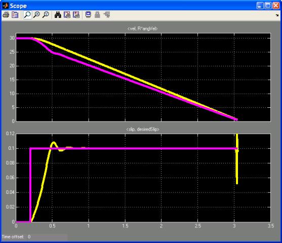
The yellow line in Figure 6 shows the vehicle longitudinal velocity and the magenta line shows the wheel’s linear velocity (calculated as the wheel radius multiplied by the angular velocity). When there is no wheel slip the two lines are the same. When the magenta line is below the yellow line there is wheel slip.

Figure 6 shows that the vehicle is initially moving forward at 30ms^-1 with no wheel slip. At T=0.2s a slip of λ = 10% is demanded, which is achieved by applying the brake to the wheel. Consequently the vehicle decelerates reducing its speed down towards zero.

The controller has the desired effect which is to track the demanded slip at the required value of 10%. It takes approximately 0.2s to achieved this level of slip, which in some applications may be too slow. In that case the controller could be redesigned to try to achieve faster tracking.

This example has demonstrated how to model a simple automotive slip control loop in Simulink. Other tutorials discussing Simulink and its applications for model based design are available on the Software Tutorials page.

Back To Top | Simulink Tutorials