Option Pricing Using The Implicit Finite Difference Method
This tutorial discusses the specifics of the implicit finite difference method as it is applied to option pricing. Example code implementing the implicit method in MATLAB and used to price a simple option is given in the Implicit Method - A MATLAB Implementation tutorial.
The Finite Difference Methods tutorial covers general mathematical concepts behind finite diffence methods and should be read before this tutorial. Alternative finite difference methods, namely the explicit method and the Crank-Nicolson method, are covered in companion tutorials.
Discretizing the Black-Scholes-Merton PDE
For the implicit method the Black-Scholes-Merton partial differential equation,

is discretized using the following formulae
- use a forward approximation
for ∂ƒ/∂t (Compare this with the
explicit method where the
backward approximation is used.)

- use a central approximation for ∂ƒ/∂S
- use a standard approximation for ∂2ƒ/∂S2


where the indices i and j represent nodes on the pricing grid.
Substituting these approximations into the PDE gives,

where

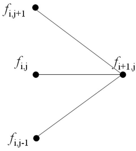
Since the equations are solved working backwards in time, superficially
Equation 1 says that three unknowns must be calculated from only
one known value.
This is shown pictorially in the following diagram,

However, when all the equations at a given time point are written simulataneously there are M-1 equations in M-1 unknowns. Hence the value for ƒ at each node can be calculated uniquely. (This can arguably be seen easier using the matrix notation shown in the following A Matrix Formulation section.)
In the option pricing framework, given the option payoff at expiry nodes then the prices Δt before expiry can be calulated, then from those prices the value 2Δt before expiry can be calculated, and working iteratively backwards through time until the option price at grid nodes for t=0 (i.e. today) can be calulated.
A Matrix Formulation
The formulation for the explicit method given in Equation 1
may be written in the matrix notation
![]()
where


and

This matrix notation is used in the Implicit Method - A MATLAB Implementation tutorial.
Stability and Convergence
Two important questions to ask about any numerical algorithm are when is it stable? and if it's stable then how fast does it converge? (An iterative algorithm that is unstable will lead to the calculation of ever increasing numbers that will at some point approach infinity. On the other hand, a stable algorithm will converge to a finite solution. Typically the faster that finite solution is reached the better the algorithm.
From standard results in matrix algebra it is known that a matrix equation of the form
given in Equation 3 is stable if and only if
![]()
Equation 4 shows the infinity norm of the matrix B -1. Heuristically, if the infinity norm of B -1 is less than 1 then successive values of Fi in Equation 3 get smaller and smaller, and hence the algorithm converges, or is stable. (Alternatively if the infinity norm of B -1 is greater than 1 then successive values of Fi get larger and larger and hence diverge.)
It can be shown that the infinity norm of B -1 is less than 1 for all values of ρ, σ and δt. Hence the implicit finite difference method is always stable. (Compare this with the explicit method which can be unstable if δt is chosen incorrectly, and the Crank-Nicolson method which is also guaranteed to be stable.)
The rate of convergence of the algorithm is directly related to the truncation error introduced when approximating the partial derivatives. Hence the implicit method converges at the rates of Ο(δt) and Ο(δS2). This is the same convergence rate as the explicit method, but slower than the Crank-Nicolson method.
A disadvantage of the implicit method is that it requires the inverse of a matrix (i.e. B -1) to be calculated, and the inverse of a matrix is (computationally) an expense operation to perform. Fortunately, for tri-diagonal matrices such as B (i.e. matrices that only have non-zero elements down their diagonal and the terms directly above and below their diagonal) fast inversion algorithms are available.
Pricing American Style Options
When pricing options that include the possibility of early exercise special care must be taken when solving Equation 3 for Fi. Taking the inverse of B to calculate a value for Fi then comparing the calculated values to the intrinsic value of the option and taking the larger value (on an element by element basis) results in incorrect option values. This is because the modified Fi will no longer satisfy Equation 3 as correct values must do.
However an iterative approach to calculating the inverse (such as the Guass-Seidel matrix inversion method) may be used successfully.