Option Pricing - Finite Difference Methods
Finite difference methods (also called finite element methods) are used to price options by approximating the (continuous-time) differential equation that describes how an option price evolves over time by a set of (discrete-time) difference equations. The discrete difference equations may then be solved iteratively to calculate a price for the option.
This tutorial covers the general mathematical concepts behind finite diffence methods. Companion tutorials cover specific aspects of the following three finite difference methods, including links to examples of implementing the methods in MATLAB,
Finite difference methods are very similar to binomial and trinomial models. The Binomial Model series of tutorials cover their use in option pricing including examples of implementing serveral versions of the binomial model in MATLAB. Other Financial Engineering tutorials may be found on the Software Tutorials page.
Each of the finite difference methods has advantages and disadvantages. However, they all involve a similar four step process. The following sections discuss those four steps,
- Discretize the appropriate (continuous-time, partial) differential equation.
- Specify a grid of potential current and future prices for the underlying asset.
- Calculate the payoff of the option at specfic boundaries of the grid of potential underlying prices.
- Iteratively determine the option price at all other grid points, including the point for the current time and underlying price (i.e. the option price today). The iteration procedure is differrent depending on whether the explicit method, implicit method or Crank-Nicolson method is being used and whether there is the possibility of early exercise of the option.
Discretizing a Differential Equation
Black, Scholes and Merton showed that a riskless
portfolio made up of an asset with value S and an option with value
ƒ(t,S) satisfies the differential equation

Equation 1 is called a partial differential equation. It is comprised of (partial) derivatives with repsect to time t and asset value S.
The solution to the Black-Scholes-Merton PDE depends on several factors, including the expected form of ƒ(t,S) and boundary conditions imposed on the solution. Boundary conditions are specified to reflect the expected payoff of the option at expiry and for minimum and maximum values of S. They are discussed in more detail in the Specifying Boundaries Conditions section.
There are several ways that the Black-Scholes-Merton PDE can be solved for the unknown value of ƒ(t,S). Black and Scholes developed an exact analytic solution for pricing plain vanilla European Put and Call options. However often an analytic solution is not available. In such instances finite difference methods can be used to calculate approximate solutions for ƒ(t,S) that are valid over small discrete time intervals Δt.
At the heart of finite difference methods are the approximation of the partial derivatives in the PDE by appropriate difference equations. Depending on the difference equations used then the explicit method, implicit method or Crank-Nicolson method is obtained.
The next sections outline different ways of approximating the partial derivatives of Equation 1.
Functions of One Variable
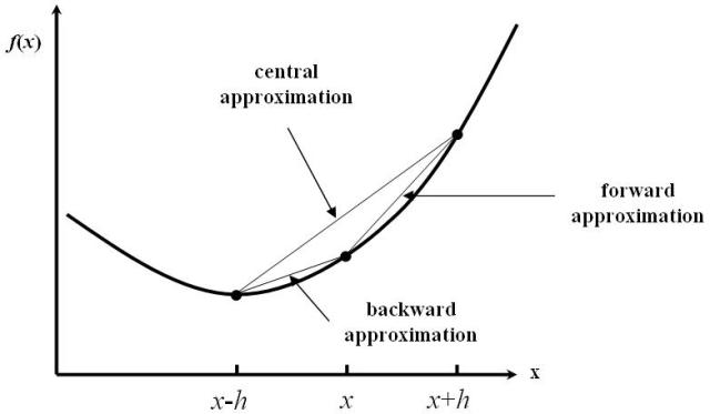
Consider the function of one variable ƒ(x) shown in Figure 1.

Then ƒ′(x), the derivative of the function at x, can be approximated in many ways. The most common are called the forward, backward and central approximation, all of which are drawn and indicated on Figure 1.
Forward Approximation
Consider the Taylor's series expansion for ƒ(x+h),

Then re-arranging Equation 2 leads to,

where Ο(h) symbolizes terms of the order of h. Assuming the step h is small then Ο(h) may be ignored and Equation 3 represents an approximation to ƒ′(x) at x.
Backward Approximation
Consider the Taylor's series expansion for ƒ(x-h),

Then re-arranging Equation 4 leads to,

where Ο(h) symbolizes terms of the order of h. Assuming the step h is small then Ο(h) may be ignored and Equation 5 represents an approximation to ƒ′(x) at x.
Central Approximation
In addition to the forward and backwards approximation there is also a central approximation
to ƒ′(x).
This is formed by subtracting Equation 4 from
Equation 2 and rearranging the result to obtain the equation,

Note that the truncation error for the central approximation is Ο(h2), i.e. of the order of h2. This implies that it converges to the correct solution faster than either the forward or backward approximations.
Approximating the 2 nd Derivative
In addition to the above first derivative approximations, to discretize the Black-Scholes-Merton PDE
of Equation 1 also requires an approxmation
for the second (partial) derivative term.
This is formed by adding the two Talyor's series approximations of Equation 2
and Equation 4 and rearranging the result to obtain the equation,

Note that as with the central approximation for the first derivative, the truncation error for this second derivative approximation is Ο(h2), i.e. of the order of h2. This has consequences for the speed of convergence of the finite difference algorithms.
Functions of Two Variables
When the function to be approximated is dependent on more than one variable (as is the case with ƒ(t,S)) and the PDE being solved contains derivatives with respect to more than one variable (as is the case with the Black-Scholes-Merton PDE of Equation 1) then the PDE is discretized by using the above approximations derived for functions of one variable while holding all other variables constant.
Specifying a Grid of Underlying Asset Prices
The second step in pricing options using a finite difference method is to create a lattice, or grid,
of potential future prices of the underlying asset(s).
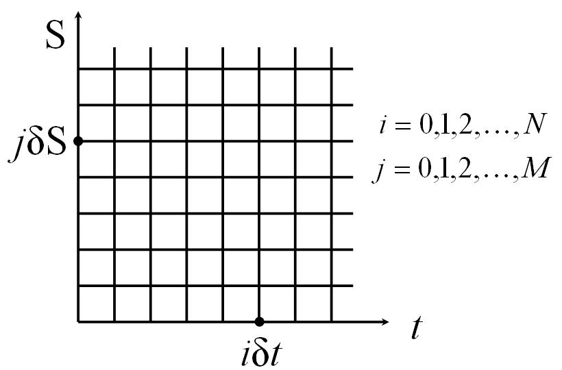
A typical grid is shown in Figure 2.

The lattice is generated by dividing the time between today and expiry into M equal periods, and the underlying price into N equal levels. This leads to a grid with M+1 time points and N+1 price levels. The grid is typically chosen so that the current price of the underlying asset lies close to the middle of the N equal price levels of the grid.
Note that time is considered to run from zero (today) to NΔt=T (at expiry). Alternative derivations may reverse this order and consider time counting down towards expiry.
Specifying Boundary Conditions
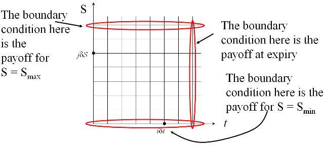
The third step in pricing options using finite difference methods is to calculate the payoff at each
node on the boundary of the grid - hence they are called boundary conditions.
The specific boundary, and the payoff for the option at the boundary, will be different
for different types of options and different parameters used in a given option.
However, a general picture is given in Figure 3.

Once the boundary conditions have been specified the interior points can be calulated using an iterative approach. The specifics of the iterative approach is different depending on the finite different method chosen and are discussed in the explicit method, implicit method and Crank-Nicolson method tutorials respectively.